

|
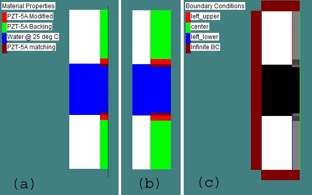
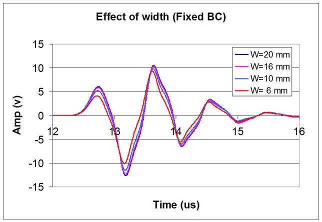
Wave2000 Plus/Wave3000 Plus for Ultrasound Transducer Design: Tutorial II (Tutorial I) In Tutorial I, simulations of transducers operating primarily in "thickness mode" were presented. When the dimensions perpendicular to the thickness become on the order of the thickness, some effects ordinarily negligible in thickness mode must be considered. In this tutorial, the 2D geometry related effects will be demonstrated using Wave2000 Plus simulations. Two typical models used in this tutorial are shown in the following figures (a) and (b). As with Tutorial I, all models of Wave2000 Plus discussed in this tutorial can be downloaded by clicking here to download Tutorial II model files. After downloading, unzip the downloaded file and copy the model files into the data folder of Wave2000 Plus. If you don't have a working version of Wave2000 Plus on your PC, a free evaluation license for Wave2000 Plus can be used to run all these models. For information of the free evaluation license for Wave2000 Plus, please click the "Download" tab above. Tips to run Wave2000 Plus models are provided at the end of this tutorial. In each model (a) and (b), there are two identical transducers working in thru-transmission mode. The one at the top is the source; the one at the button is the receiver. Water fills the space between the two transducers. The transducers have three components: a piezoelectric layer (2 mm thick x W mm wide) made of PZT-5A, a backing layer (20 mm thick x W mm wide) and a matching layer (1 mm thick x W mm wide). Six Ws (widths) are used to demonstrate the effect of width on the received signal.In the above figure, W = 6 mm (a) and W = 16 mm (b). For all models in this tutorial, the input signal is a 1 volt pulse with duration 0.1 us. The receiver output is recorded by Wave2000 Plus with a 60 dB gain. Another aspect to be simulated in this Tutorial II is related to the boundary conditions. In Tutorial I, it was assumed that the three layers are bonded to a rigid shell; this boundary condition is simulated using a fixed boundary as shown in above figure (c) (i.e., the thin red and blue lines on the left side of the matching, piezoelectric and backing layers, of the source and receiver transducers, respectively). In addition to the fixed BC, in this Tutorial II the free boundary conditions are also simulated to demonstrate the effect of boundary condition on the received signals. Again Wave2000 Plus is used to simulate the models; however, analogous models can be used in 3D with Wave3000 Plus. Since plane strain is used in Wave2000 Plus, the geometry of simulated transducers has a dimension perpendicular to the screen (depth) much bigger than both its height (thickness) and width. Due to the symmetry of the geometry and boundary condition, only half of the model needs to be simulated by constraining no horizontal displacement in the center (see the thin green line in the figure above (c)). The effects of width and boundary condition on wave signal are demonstrated using the Wave2000 Plus models. Effect of Piezoelectric Element/Backing/Matching Widths: When the width W of a transducer is reduced, the energy output of a transducer is also reduced. In addition, the shape of the wave signal also changes. In particular, when the width and height are close to one another, the 2D effect (i.e., not pure "thickness mode") needs to be included in modeling and designing such a transducer. The following two figures present the received potential from the simulations for 6 different widths with the fixed boundary condition. The input signal is a one-volt pulse with a 0.1 us time duration. The element widths simulated are 20, 16, 10, 6, 2 and 1 mm.
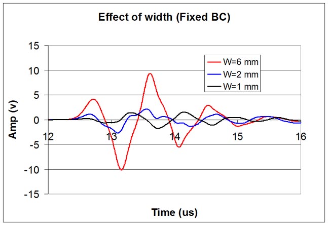
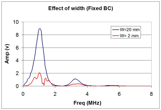
The figures show the received potentials are approximately the same when the transducer's width is more than 10 mm. The figures also show that as the width becomes smaller, the received potential is reduced, but perhaps more importantly is that the shape of the wave signal changes significantly. When the transducers' widths are 10 mm or more, the received potentials are relatively smooth. When the transducers' widths are small, the shape of the received voltage signals are no longer smooth, which may indicate multiple frequency components/modes are included. To demonstrate this, the amplitude spectra of the voltage outputs of models with widths equal to 20 and 2 mm are plotted in the following figure.
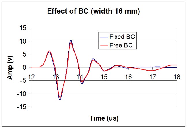
The above figure clearly shows the spectra of model of width 2 mm has multiple frequency components. In cases like this, the effect of the 2D geometry must be considered in designing transducers. Effect of Boundary Conditions The characteristic of a vibrating system is highly dependent on the boundary conditions. Usually a transducer is sealed in a solid shell, therefore some kinds of constraints are typically applied to the active element, and backing and matching layers. To demonstrate the effect of boundary conditions on a transducer, two extreme boundary conditions are used in this Tutorial II. One set of conditions is a fixed boundary condition, while the other set is a free boundary condition. The following two figures show the effect of these two boundary conditions on the received voltage outputs, for a relatively wide transducer element (16 mm wide) and a relatively narrow transducer element (2 mm wide); remember that all these simulations are carried out with 2 mm thick piezoelectric elements.
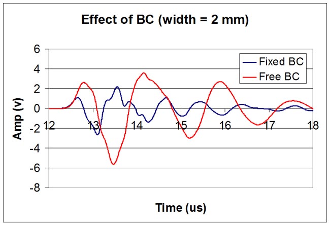
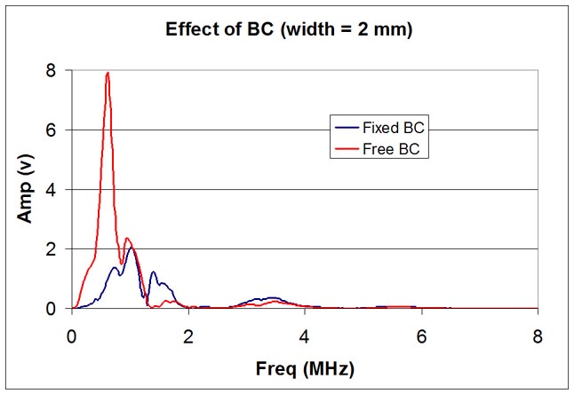
In the first figure, the width is 16 mm and as may be seen there is little effect on the early (main) portion of the received signal of the boundary condition. However, a difference between the two signals may be seen to begin at about 16 us, where the free BC model shows a low frequency signal while the fixed BC does not. This presumably is due to the presence of a multi-mode signal that arises in the case of the free BC. In the bottom figure, the piezoelectric element width is 2 mm. The effect of boundary condition is clearly demonstrated. Except for the earliest (rising) portion of the received signals, the two outputs have little in common. Presumably, both signals being highly multi-mode, are both affected by the two distinct BCs. The difference between the two BCs can also be presented in the frequency domain, as the following figure shows.
Summary: The effects of geometry and boundary condition have been demonstrated using Wave2000 Plus. The simulations show the aspect ratio of a transducer and boundary condition can affect the characteristics of the transducer greatly, especially when the width and height of the elements are of the same order. The models used are all two dimensional, which can approximate the cases where the third dimension is much larger than the dimensions considered. If however, the third dimension is comparable to the two dimensions considered in Tutorials I and II, 3D models need to be used to accurately simulate the 3D effects. As Wave2000 Plus can be used to simulate 2D models, Wave3000 Plus can be used to simulate 3D models. A free evaluation license for Wave3000 Plus can be used to run 3D models. For information on the free evaluation license for Wave3000 Plus, please click the "Download" tab above. Tips for running the Wave2000 Plus models: (1) To calculate the spectrum of receiver output signal, after completing a simulation, use menu command Analysis->Spectrum Plot. To customize the plot, double click anywhere inside the plot window to display a plot dialog. To export the plotted data to a file, click on "Export" button, then choose a file to save.
Go to Tutorial I
|
|||||||||
© 2024 CyberLogic, inc. All Rights Reserved